Filtering a signal means removing out the unwanted frequencies from signal while preserving the desired frequencies. One application of filtering is removing the noise from a signal. Digital filters are polynomial functions that does the wave-shaping of the signal. In this article we will see the overview of FIR filters, Linear Phase FIR filters and type of FIR filters.
Here we will cover the outline and things to be taken care before implementing a filter type. Again these tutorials do not cover the theoretical aspect in depth. Here we focus on the implementation of the filters.
Filters
A filter generally has a pass band, transition band and a stop band. Look at the figure. This is an example ideal low pass filter.
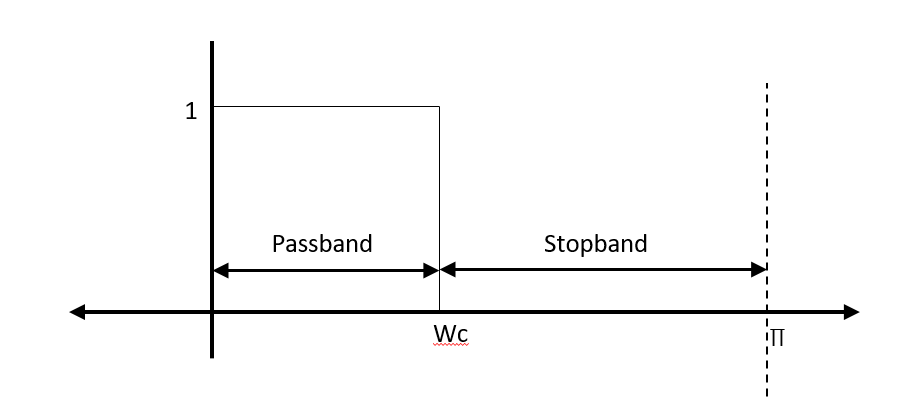
This filter is represented by h(n). In the design of a filter, we want a polynomial function ‘h(n)‘ which when applied to the input signal ‘x(n)‘ will produce a filtered output ‘y(n)‘.

FIR Filters
The FIR filters are the class of filters that have a finite duration impulse response. These filters are inherently stable. The general FIR filters have transfer function of type
One can observe that these filters have no feedback element. If we take the z transform of such filter then the transform would have only zeros and no poles. This is an important characteristic of FIR filter.
Linear Phase FIR Filters
Linear phase filters are those filters whose phase response varies linearly with frequency. Each of the frequency component of the signal is delayed by a constant amount. Hence such filters preserve the shape of signal and introduce no distortions. This is an important characteristic required for some applications which cannot tolerate phase distortions at all.
For a filter to be linear phase, it must have
There are four types of linear phase FIR filters-
| Filter Length | Symmetric / Anti | Impulse Response | Type |
| Odd | symmetric | h(n) = h(M-n) | 1 |
| Even | symmetric | h(n) = h(M-n) | 2 |
| Odd | anti-symmetric | h(n) = -h(M-n) | 3 |
| Even | anti-symmetric | h(n) = -h(M-n) | 4 |
Note: M is order of filter. Order of filter = length of filter – 1
The location of zeros is important and is used to design the filters.
Type 1 Linear Phase FIR Filters
Type 1 filters have the odd length and is symmetric around middle sample.
This filter have frequency response of type –
Above equation simply means coefficient of filters are symmetric about some middle sample. I’ll refrain myself from writing above such equation. This was just to show the frequency response notation. From the pole and zero of z-transform of type 1 filters –
- There can be either no zeros or even number of zeros at z = 1 or z = -1
- If zeros are purely real or imaginary, not on unit circle, then they appear in pairs.
- If zeros are complex, and not on unit circle, they occur in quadruple
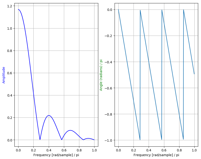
Here is an example – we have drawn a filter having coefficients – [0.5, 1, 1, 1, 1, 1, 0.5]
One can notice that this is odd length – symmetric filter.

Notice from the phase diagram that phase linearity is piece-wise linear.
This filter has zero calculated as-
zeros: [ 0.6234898 +0.78183148j 0.6234898 -0.78183148j -0.22252093+0.97492791j
-0.22252093-0.97492791j -0.90096887+0.43388374j -0.90096887-0.43388374j
-1. +0.j ]
On calculating the zeros of the z-transform of the filter one can see that this filter has zeros a pair of zeros at z = 1 and no zeros at z = -1. This satisfies requirements for type 1 filter.
TYPE 2 LINEAR PHASE FIR FILTERS
Type 2 filters have the even length. Because of even length, they are symmetric around imaginary axis.
For such filters, it is mandatory to have an odd number of zero at z = 1 and even or no zeros at z = -1. The zero at z= – 1 also imposes restriction on its design for High Pass filter.
We have implemented an 8 length filter to show this. this filter has coefficient as [0.5, 1, 1, 1, 1, 1, 1, 0.5].
Also this filter is symmetric about imaginary axis. The zeros calculated for such a filter is –
zeros: [ 0.6234898 +0.78183148j 0.6234898 -0.78183148j -0.22252093+0.97492791j
-0.22252093-0.97492791j -0.90096887+0.43388374j -0.90096887-0.43388374j
-1. +0.j ]
We can see that there is one zero at z = -1 and no zeros at z=-1. This satisfies above requirement.
TYPE 3 LINEAR PHASE FIR FILTERS
Type 3 filters have the odd length and is anti-symmetric around middle sample.
For type 3 filters, it is mandatory to have a odd number of zero at z = 1 and z = -1. And middle sample value is 0.
Because of the presence of the zeros at z = -1 and z= 1 these filters can only be used to design band pass filters. They do not allow low and high frequencies to pass through.
Filter implementation with filter coefficients [0.5, 1, 1, 0, -1, -1, -0.5] is being shown in figure.
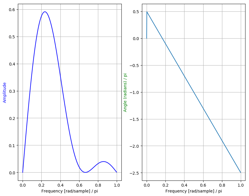
The zeros calculated for such a filter is
zeros: [-1. +0.j 1. +0.j -0.5+0.86602542j -0.5-0.86602542j -0.5+0.86602539j -0.5-0.86602539j]
One can notice that it has zeros at z = 1 and z = -1. This is one of the requirements for low type 3 filter.
TYPE 4 LINEAR PHASE FIR FILTERS
Type 4 filters have even length and is anti-symmetric around middle sample.
For type 4 filters, it is mandatory to have a odd number of zero at z = 1 and odd or no zeros at z = -1.
Because of the presence of the zeros at z= 1 these filters cannot be used to design low pass filters.
Filter implementation with filter coefficients [0.5, 1, 1, -1, -1, -0.5] is being shown in above figure.

Zeros calculated for the above filter is
zeros: [-1.12174441+1.3066224j -1.12174441-1.3066224j 1. +0.j -0.37825559+0.440597j -0.37825559-0.440597j ]
This filter also has a zero present at z=1.
Sample Code-
Following is the python code for showing various types of the filter.
We have use python’s signal.tf2zp to plot signals. Also the frequency response is shown from 0 to pi. We have not shown how to design such filters, This will be covered in upcoming articles.
For type 1 filter the code is shown below.
# -*- coding: utf-8 -*-
"""
Created on Tue Oct 15 11:06:45 2019

@author: irawat
"""

import numpy as np
import matplotlib.pyplot as plot
from scipy import signal

#""""
#For linear phase, the impulse response must satisfy -
#h[n] = +-h[M-n]
#H(z) = +-z**-M . H(z**-1)
#""""


# Type 1 linear phase FIR filter
# sequence is symmetric and of odd length
# for symmetric filter h[n] = +h[M - n]
# H(w) = exp(-jw M/2){ h[M/2] + 2 * sum(i: (1, M/2), h(M/2 - i).cos(wi) ) }
# Phase = -wM/2 + b,
# for type 1 filters, there can be either no zeros or even number of zeros at z = 1 or z = -1

# e.g. consider M = 6; 7 length FIR filter
# h(n) = 1/6[0.5, 1, 1, 1, 1, 1, 0.5]
# on solving
# |H(w)| = 1/6.h[3] + 2.h[0]cos(3w) + 2.h[1]cos(2w) + 2.h[2]cos(w)
# arg = -w3 + b
# plot this signal for magnitude and frequency

filCoeff = np.array([0.5, 1, 1, 1, 1, 1, 1, 0.5])
filCoeff = filCoeff / 6

# filter
w, h = signal.freqz(filCoeff,a=1)

# angle
angles = np.unwrap(np.angle(h))

#plot - magnitude
plot.subplot(121)
#plot.plot(w/np.pi, 20 * np.log10(abs(h)), 'b')
plot.plot(w/np.pi, abs(h), 'b')
plot.xlabel('Frequency [rad/sample] / pi')
#plot.ylabel('Amplitude [dB]', color='b')
plot.ylabel('Amplitude', color='b')
plot.grid(which='both')

plot.subplot(122)
plot.plot(w/np.pi, angles/np.pi)
plot.grid(which='both')
plot.ylabel('Angle (radians) / pi', color='g')
plot.xlabel('Frequency [rad/sample] / pi')
plot.show()

# pole and zeros of filter -
zeros, poles, gain = signal.tf2zpk(filCoeff, 1)

print("zeros:", zeros)
print("pole:", poles)
print("gain:", gain)

# filter plot -
x =  np.arange(-4, 4)
plot.stem(x, filCoeff * 6)
plot.grid(which='both')
plot.ylabel('x[n]')
plot.xlabel('bins')
One can replace the filter coefficient for the type of filter he wants to implement.
And that’s it for now. Next we will know bout speech signals so that we may apply some of the filter principals far to something interesting.
Also I want to point out, instead of viewing the absolute amplitude of the signal, one should use dB scale for more sense. The -3 dB point in such representation will represent the half power point. This is the point where cutoff frequency of the filter is located.
Thanks.
