In the first tutorial we saw how to draw a signal of given frequency. In this tutorial we will see how to observe the spectrum of a signal.
We know to draw a sinusoidal signal we need two information : frequency of the signal and sampling frequency. Also Nyquist rule has to be respected. But what if we had a random signal and we want to know if certain frequency is present in the signal or not?
The Discrete Fourier transform (DFT) is the exact transform that does this. It takes the signal and finds all the frequencies contained in the signal.
Since DFT is a vast topic we are not covering it’s theoretical aspect in depth. One must refer textbooks for in depth understanding of DFT. We will keep our discussion concise and focus on the implementation and interpretation of DFT.
Mathematically DFT is given by:
Here N is duration of the signal.
The transform is also of duration N. i.e. {k = 0, 1, … N – 1}, and is periodic w.r.t. N.
For finding DFT, we assume signal duration is finite.
For infinite signals, we take a portion of signal and calculate its transform (we will see further how to deal with long duration signals in Windowing).
Points to keep in mind before moving further –
1. DFT is actually a complex quantity, i.e. each of the X(k) is actually a complex number. Hence we have to magnitude of the complex number.
2. The DFT samples found for k > N/2 is of no practical significance. (Find out why, Hint: conjugate property, X[k] = X*[-k])
3. In the transformed samples, first N/2 samples have all the frequencies present up-to (sampling frequency ‘fs’ / 2). This also mean that we cannot observe frequencies more than fs / 2. We are not interested anyways as we respect Nyquist.
Example-
Let’s calculate a DFT of a signal.
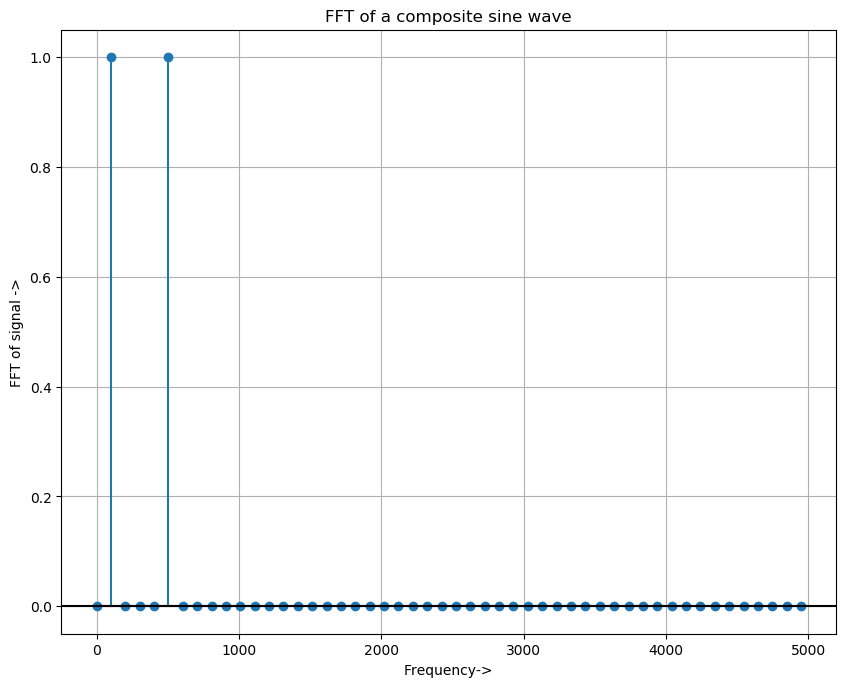
Let’s draw a signal consisting of two components of signal of 100 Hz (fm1 = 100 Hz) and 500 Hz (fm2 = 100 Hz) signal. Our signal duration will be 100 samples, i.e. N = 100. Also let’s take sampling frequency as 10000 Hz (fs = 10000).
We want to find the frequency specturm. To find the DFT, there is an algorithm called FFT (Fast Fourier Transform). FFT is very fast and efficient in finding DFT. To find N point DFT, we use Python’s FFT algorithm.
import numpy as np
import matplotlib.pyplot as plot

numSamples = 300

# ----------------------------------------------------------
# sine wave of 100 Hz and 500 Hz, sampling freq 10000 Hz

fs  = 10000.0
fm1  = 100.0
fm2 = 500.0

time        = np.arange(0, numSamples, 1);
amplitude   = np.sin(2 * np.pi * fm1 / fs * time)
amplitude2  = np.sin(2 * np.pi * fm2 / fs * time)
aplitude_result = amplitude + amplitude2

# plot.plot(aplitude_result)
# plot.show()

# ----------------------------------------------------------
# FFT of signal
# Number of samplepoints

numPoints = numSamples
fftSignal = np.fft.fft(aplitude_result, numPoints)
xf = (fs/2) / numPoints * np.linspace(0, numPoints - 1, numPoints/2)
plot.stem(xf, 2 / numPoints * np.abs(fftSignal)[0:numPoints//2])

# Give x axis label for the sine wave plot
plot.title('FFT of a composite sine wave')
plot.xlabel('Frequency->')
plot.ylabel('FFT of signal ->')
plot.grid(True, which='both')
plot.axhline(y=0, color='k')
plot.show()
Result interpretation –
- We have calculated ‘N’ point DFT. Each of the element of the array is complex a complex number.
- The real part of the sample are from the even parts of the signal and imaginary parts are from the odd parts of the signal.
- In the image, each of the sample is actually magnitude of the complex number. (If squared and plotted, this will be called power spectrum.)
- Only half of the samples are drawn in the image. That coves all the frequencies upto fs / 2.
Resolution –
The difference between two successive frequency samples defines the resolution of FFT.
We know FFT covers frequencies upto fs / 2, so each of the gap is (fs / 2) / N apart.
(Note that these are discrete numbers, so if our sample frequency falls in between two DFT samples, it will be redistributed to nearby samples. )
That’s why if we use higher number of N, better is the frequency resolution. But again, more is the computation.
In our example, each sample is 100 Hz apart. that’s why there are two peaks at second sample for 100 Hz and at 6th sample for 500 Hz.
Windowing
Above we saw a finite short duration signal N=100. There was not much difficulty in finding the FFT. But what if our signal is long duration or say online, we can’t wait for that long. Also if signal is a long duration, the calculation for FFT also increases.
We said that for such signals, we extract a portion of signal and find the transform. Continuing with that discussion, If we extract a portion of signal directly, this is like sudden termination of signal at the edges.
The sudden discontinuity in signal distorts the spectrum of signal. To counter this, the signal has to multiplied with a window function. This is called windowing. By doing this operation, we minimize the distortions in the signal. There are a number of windowing functions available. With each having its own merits. Based on the requirements we can choose the correct window function.
Consider the following example. We have again considered a composite signal from above but the signal is of longer duration. In the first image we have applied a rectangular window to the signal. Then we calculated FFT for the portion of signal where window was applied. Look how the spectrum gets distorted. This is because of the abrupt termination at the edges of the rectangular window.
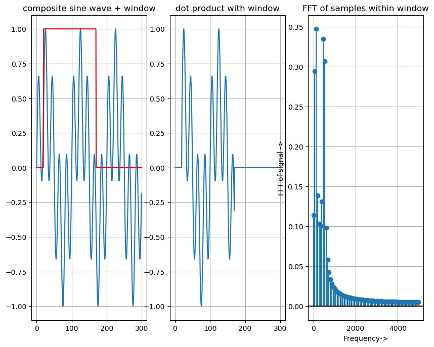
In the second example we have applied sine window to the signal, see its effect on the signal’s spectrum. The envelope of the sine window is shown with red color. See how spectrum of signal

Python code to demonstrate windowing effect-
import numpy as np
import matplotlib.pyplot as plot

numSamples = 300

# ----------------------------------------------------------
# sine wave of 100 Hz and 500 Hz, sampling freq 10000 Hz

fs  = 10000.0
fm1  = 100.0
fm2 = 500.0

time        = np.arange(0, numSamples, 1);
amplitude   = np.sin(2 * np.pi * fm1 / fs * time)
amplitude2  = np.sin(2 * np.pi * fm2 / fs * time)

aplitude_result = amplitude + amplitude2
aplitude_result /= np.max(np.abs(aplitude_result), axis=0)

windowSize = 150
windowStart = 20
window = np.zeros(numSamples)

# ----------------------------------------------------------
## for rectangular window comment next section and uncomment this section
# form a rect window
window[windowStart:windowSize + windowStart] = 1

# ----------------------------------------------------------
## for sine window comment previous section and uncomment this section
## form a sine window
#n = np.arange(0, windowSize, 1)
#sineWindow = np.sin(np.pi * n / windowSize)
#windowSize = 150
#windowStart = 20
#window[windowStart:windowSize + windowStart] = sineWindow
# ----------------------------------------------------------
# draw first
plot.subplot(1,3,1)
plot.plot(aplitude_result)
plot.plot(window, color='r')
plot.grid(True, which='both')
plot.title("composite sine wave + window")


# ----------------------------------------------------------
# FFT of long signal
# Number of samplepoints
portion_signal = window * aplitude_result

plot.subplot(1,3,2)
plot.grid(True, which='both')
plot.title("dot product with window")
plot.plot(portion_signal)


# ----------------------------------------------------------
portion_signal = portion_signal[windowStart:windowSize + windowStart]
numPoints = windowSize
fftSignal = np.fft.fft(portion_signal, numPoints)
xf = (fs/2) /  numPoints * np.linspace(0, numPoints - 1, numPoints/2)

plot.subplot(1,3,3)
plot.stem(xf, 2 / numPoints * np.abs(fftSignal)[0:numPoints//2])
plot.title('FFT of samples within window')
plot.xlabel('Frequency->')
plot.ylabel('FFT of signal ->')
plot.grid(True, which='both')
plot.axhline(y=0, color='k')
plot.show()
We lose the information in signal because of the shape of the window. To overcome this we use overlapped windows. Do explore on that. Windowing is an important concept.
Moreover windowing technique is also used for designing sub-optimal filters. One can explore more on windowing by applying different window functions and observe it’s effect.
That’s it! Thanks.
